Plotting Wind Properties

As described under Models, Python saves wind properties in binary wind_save files. This notebook explains how to read and plot wind variables for the cv_standard file found in the examples. Before running the python commands, you need to run the model from the command line. I suggest running the following commands, after you have compiled python:

mkdir cv_test
cd cv_test
cp $PYTHON/examples/basic/cv_standard.pf .
py cv_standard </code>

The model will take about 5 minutes to run on a single core. It will not converge, but will give us a model to use as an example. You should then run windsave2table on the output

windsave2table cv_standard

which will create a series of ascii files containing key variables in the wind cells. We will use these ascii files for our plots.

Make A Basic Quick Look Wind Plot

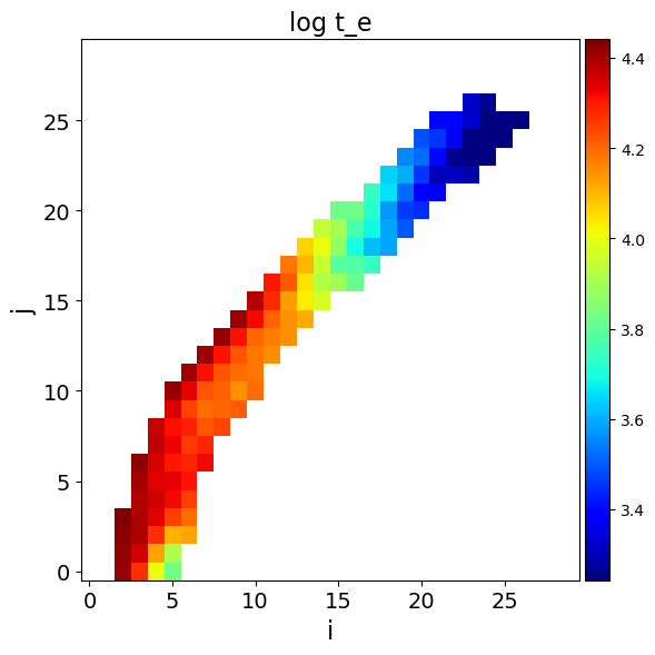
The simplest way to make a quick look plot of the electron temperature is using the plot_wind.py routine in $PYTHON/py_progs. In this example, I will assume py_progs has been added to $PATH and to $PYTHONPATH. plot_wind.py can be run from the command line using

plot_wind.py cv_standard t_e

where the second argument is the variable to plot. Alternatively, it can be run from within a python script by doing (where we are now assuming you are running this code from one directory above cv_test):

%matplotlib inline
import matplotlib.pyplot as plt
import numpy as np
import plot_wind
fname = "cv_test/cv_standard.master.txt"
plot_wind.doit(fname, var="t_e")

'cv_test/cv_standard_log_t_e.png'

More detailed/customisable plots

You may, however, wish to get more direct access to the data, which can be done easily by reading in the cv_standard.master.txt file, for example using astropy. In the next code block, we read in the data file and print out the columns.

import matplotlib.pyplot as plt
import astropy.io.ascii as io

data = io.read(fname)

print (data.colnames)

['x', 'z', 'xcen', 'zcen', 'i', 'j', 'inwind', 'converge', 'v_x', 'v_y', 'v_z', 'vol', 'rho', 'ne', 't_e', 't_r', 'h1', 'he2', 'c4', 'n5', 'o6', 'dmo_dt_x', 'dmo_dt_y', 'dmo_dt_z', 'ip', 'xi', 'ntot', 'nrad', 'nioniz']

The py_plot_util script in py_progs comes with a handy guide to the main columns in the .master.txt file and returns a dictionary containing the description for all variables.

import py_plot_util as util
descr = util.get_windsave_descriptions(data)

no description for column x
z          --  left-hand lower cell corner z-coordinate, cm
xcen       --  cell centre x-coordinate, cm
zcen       --  cell centre z-coordinate, cm
i          --  cell index (column)
j          --  cell index (row)
inwind     --  is the cell in wind (0), partially in wind (1) or out of wind (<0)
converge   --  how many convergence criteria is the cell failing?
v_x        --  x-velocity, cm/s
v_y        --  y-velocity, cm/s
v_z        --  z-velocity, cm/s
vol        --  volume in cm^3
rho        --  density in g/cm^3
ne         --  electron density in cm^-3
t_e        --  electron temperature in K
t_r        --  radiation temperature in K
h1         --  H1 ion fraction
he2        --  He2 ion fraction
c4         --  C4 ion fraction
n5         --  N5 ion fraction
o6         --  O6 ion fraction
dmo_dt_x   --  momentum rate, x-direction
dmo_dt_y   --  momentum rate, y-direction
dmo_dt_z   --  momentum rate, z-direction
ip         --  U ionization parameter
xi         --  xi ionization parameter
ntot       --  total photons passing through cell
nrad       --  total wind photons produced in cell
nioniz     --  total ionizing photons passing through cell

py_plot_util also contains some routines for reshaping and masking arrays and so on. One of the most useful for plotting is the wind_to_masked function which turns the raw 1D flattened data into a masked 2D array with the right shape which can be easily used with pcolormesh and so on. Here’s an example plot of the electron density in the model.

x, z, ne, inwind = util.wind_to_masked(data, value_string="ne", return_inwind=True)
plt.pcolormesh(x,z, np.log10(ne))
plt.loglog()
plt.xlim(1e9,1e12)
plt.ylim(1e8,1e12)
cbar = plt.colorbar()

/Users/matthewsj/.mpi_temp/ipykernel_31972/816639112.py:2: RuntimeWarning: divide by zero encountered in log10
  plt.pcolormesh(x,z, np.log10(ne))

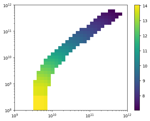
This procedure can be used to plot any of the variables in the masterfile and is a good starting point for delving into the properties of the wind.

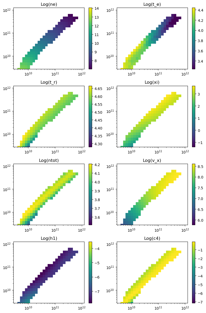
To make a simple multi-panel plot of wind properties, you can use some of the routines in py_plot_output. The example below plots all the variables passed in an array and saves the file as cv_standard_wind.png

import py_plot_output as plot
plot.make_wind_plot(data, "cv_standard_wind", var = ["ne", "t_e", "t_r", "xi", "ntot", "v_x", "h1", "c4"], shape=(4,2) )

/Users/matthewsj/opt/anaconda3/lib/python3.9/site-packages/astropy/table/table.py:3474: FutureWarning: elementwise == comparison failed and returning scalar instead; this will raise an error or perform elementwise comparison in the future.
  result = self.as_array() == other
/Users/matthewsj/winds/python/py_progs/py_plot_output.py:301: RuntimeWarning: divide by zero encountered in log10
  p.pcolormesh(x,z,np.log10(v))

7363719978102.189
12772.992700729927
37305.83941605839
1214.8115635036497
11854.087591240876
145555532.84671533
5.267621167883212e-06
0.41242660718248175

0

Plotting Ion Populations

Ion populations outputted from windsave2table are stored in files like cv_standard.C.frac.txt, where the letter before frac denotes the element. Plots of the C III ion fraction can thus be made through commands like the following, where strings like i05 index the ion for each file.

carbon_ion = io.read("cv_test/cv_standard.C.frac.txt")
x, z, c3_frac, inwind = util.wind_to_masked(carbon_ion, value_string="i03", return_inwind=True)
plt.pcolormesh(x,z, np.log10(c3_frac))
plt.loglog()
plt.xlim(1e9,1e12)
plt.ylim(1e8,1e12)
cbar = plt.colorbar()

/Users/matthewsj/.mpi_temp/ipykernel_31972/4163463376.py:3: RuntimeWarning: divide by zero encountered in log10
  plt.pcolormesh(x,z, np.log10(c3_frac))